Arima Model for Forecasting: A Comprehensive Guide to Time Series Prediction

Understanding ARIMA Model

ARIMA (Auto Regressive Integrated Moving Average) is a powerful time series forecasting model. This model is widespread for its compliance, ARIMA excels in capturing complex time series patterns, exceptionally in data featuring trends and seasonality. Analysts influence ARIMA to extract insights from historical data and predict future consequences across numerous domains, including finance, economics, and sales forecasting. Its simplicity, interpretability, and versatility make it an ideal preference for modelling complicated chronological dynamics and granting precise forecasts.

Definition of Arima Model

The ARIMA (Auto-Regressive Integrated Moving Average) model is an extensively used statistical method for analysing and forecasting time series data. It combines three important components like autoregressive (AR), differencing (I), and moving average (MA). These components bestow a adaptable framework for modelling and forecasting time series data across numerous domains.

Importance of ARIMA Model in Forecasting

The ARIMA (Auto-Regressive Integrated Moving Average) model holds significant importance in forecasting for several reasons:

1. Flexibility: ARIMA is a versatile model capable of capturing a wide range of time series patterns, including trends, seasonality, and irregular fluctuations. Its flexibility makes it applicable to various types of data across different domains.
2. Interpretability: The components of the ARIMA model (autoregressive, differencing, moving average) have clear interpretations, allowing analysts to understand the underlying dynamics of the time series data and interpret the results of the forecasting model.
3. Forecast Accuracy: ARIMA models are effective in generating accurate forecasts, particularly for short-to-medium-term predictions. By capturing the patterns and relationships within the data, ARIMA can provide valuable insights into future trends and behaviours.
4. Data-driven Decisions: The forecasts generated by ARIMA models enable data-driven decision-making in various fields such as finance, economics, marketing, and operations. Businesses and organizations can use ARIMA forecasts to optimize resource allocation, plan inventory levels, and make strategic decisions.
5. Diagnostic Tools: ARIMA models offer diagnostic tools such as autocorrelation and partial autocorrelation functions, which help analysts assess the model’s adequacy and identify any deficiencies that need to be addressed.

Components of ARIMA Model

Autoregressive Aspect (AR)

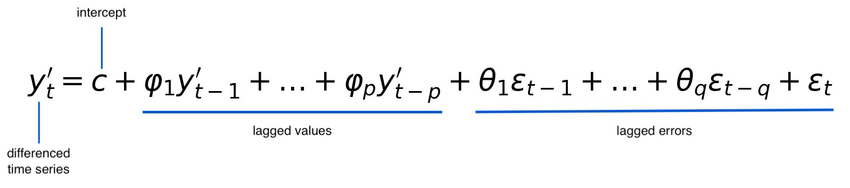
Autoregression refers to a regression of the variable against itself, with the key idea being that the current value of a time series can be expressed as a linear combination of its previous values. The AR component is characterized by its order, denoted as “p”. This represents the number of lagged observations included in the model. For example, AR(p) indicates that the current value of the time series depends on the previous “p” values. Estimating the parameters (coefficients) of the autoregressive model involves techniques such as ordinary least squares (OLS) regression or maximum likelihood estimation (MLE).

Integrated Component (I)

Designed to ensure stationarity in the time series data. The integrated component addresses non-stationarity by differencing the time series data. Differencing involves computing the difference between consecutive observations to remove trends or other systematic patterns. The order of differencing, denoted as “d”, represents the number of times differencing is applied to achieve stationarity. : The order of differencing “d” is determined by the number of times differencing is required to make the data stationary.

Moving Average Part (MA)

The MA component models the relationship between an observation and a residual error from a moving average model applied to lagged observations. It accounts for the influence of random shocks or innovations on the current value of the time series. Similar to the autoregressive component, the MA component is characterized by its order, denoted as “q”. This represents the number of lagged forecast errors included in the model. For example, MA(q) indicates that the current value of the time series depends on the “q” most recent forecast errors.

Practical Application of ARIMA Model

BITCOIN: A Case Study

Bitcoin, as a digital currency, has attracted significant attention from investors, researchers, and analysts alike. Analysing Bitcoin prices using time series forecasting methods like the ARIMA model provides insights into its price movements and aids in predicting future trends. Let us delve into a case study related to the ARIMA model and time series forecasting for Bitcoin and analyse its performance in predicting future price movements.

Importing the Libraries

Essential Python libraries for financial data analysis and time series modelling. pandas and numpy are used for data manipulation and numerical computing, while matplotlib.pyplot facilitates data visualization, yfinance are employed to fetch historical market data, particularly from Yahoo Finance. The statsmodels library is utilized to fit ARIMA models to time series data, and scikit-learn’s mean_squared_error function evaluates model performance. Datetime manipulates dates and times, and warnings filterwarnings ignores any potential warnings during code execution. Overall, these libraries form the foundation for conducting comprehensive analysis and forecasting in the realm of financial data.

Importing the Dataset

The “yfinance” or “yf” library in Python provides a convenient means to access historical market data, encompassing stock prices, dividends, and granular information sourced from Yahoo Finance. This versatile tool offers flexible access to financial data across various asset classes, including stocks, exchange-traded funds (ETFs), and indexes, facilitating comprehensive analysis and research endeavours.

Checking Missing Values

In streamlining the dataset, our objective was to enhance its simplicity and optimize the model’s performance. Specifically, we opted to exclude non-essential columns, such as ‘Close’, while retaining ‘Adj Close’ for analysis. This deliberate selection aims to refine our modelling strategy for improved accuracy. 

Notably, the dataset demonstrates a lack of missing values, reflecting its comprehensive and well-rounded nature. As such, there is no need for imputation techniques, reaffirming the dataset’s integrity and suitability for further analysis.

Correlation Map

Our objective was to explore the interrelationships between different aspects of our dataset and the focal variable of interest, namely, “Adj Close” prices. Through correlation analyses, we identified strong associations between attributes like ‘High’ and ‘Close’ with ‘Adj Close’ prices. Conversely, ‘Volume’ demonstrated a relatively weaker impact. This observation aids in understanding how changes in particular features might affect our forecasts for ‘Adjusted Close’ values, contributing to a comprehensive grasp of the data dynamics

Creating New Data Frame for ARIMA model

A new Data Frame was constructed with the columns “Date” and “Adj Close” to meet the requirements of the ARIMA model. This ensures compatibility with ARIMA input structure, facilitating accurate and efficient modelling and forecasting processes.

Reindexing the New Data frame and Plotting Seasonal Components

Reindexing was performed to facilitate the visualization of time series forecasting components. The ‘Date’ column was designated as the primary index against the ‘Adj Close’ column, ensuring that each observation aligns with its corresponding date stamp. This restructuring allows for straightforward plotting and analysis of time series components, enabling a clear understanding of trends, seasonality, and other patterns within the data.

Standardising the New Data Frame

Standardization was implemented to enhance the interpretability of values and to improve the accuracy of forecasts. By standardizing the data, we transform it into a common scale, ensuring that all variables have a mean of zero and a standard deviation of one. This process facilitates easier comparison and mapping of values across different features. Additionally, standardization helps stabilize model performance by preventing features with larger scales from dominating the analysis. Ultimately, standardization aids in generating more accurate forecasts by promoting consistency and reducing the impact of outliers or extreme values.

Auto Arima

Auto ARIMA was executed to determine the optimal values of the parameters p, d, and q for the ARIMA model. This automated process searches through various combinations of parameters and selects the one that yields the best model performance based on predefined criteria such as Akaike Information Criterion (AIC) or Bayesian Information Criterion (BIC). The value we got of p, d, q are 1, 0, 0 respectively. It was done in order to choose the correct order of ARIMA.

Splitting of the Dataset

The dataset was partitioned into training and testing sets testing data consist of past 1 year data that is 365 data points and training set has remaining data. This division allows for the evaluation of model performance on unseen data. The training set is used to fit the model, enabling it to learn patterns and relationships within the data. Subsequently, the model’s performance is assessed on the testing set, providing an indication of its ability to generalize to new observations.

Implementing Arima 

The model to fit the training set of ‘Adj Close’ prices. Configured with an order of (1, 0, 0) for the ARIMA components and a seasonal order of (2, 1, 0, 12), indicating seasonal AR components of order 2, seasonal differencing of order 1, and no seasonal MA components with a period of 12. Through the fit() method, the model is trained on the training data to estimate parameters, yielding a ‘result’ object. The summary() facilitates assessment of the model’s performance and the significance of each parameter in capturing the temporal patterns inherent in the ‘Adj Close’ prices time series.

Forecasting using ARIMA Model

After fitting the SARIMAX model to the training data, it is subsequently employed for forecasting, which constitutes a pivotal aspect of time series analysis. Forecasting involves predicting future values of the time series based on historical data and the estimated model parameters. By leveraging the trained SARIMAX model, we can generate forecasts for ‘Adj Close’ prices over the forecast horizon.

Real World Use-Cases of ARIMA Model

1. Financial Forecasting: ARIMA predicts stock prices, exchange rates, and financial indicators, aiding investment decisions.

1. Demand Forecasting: ARIMA forecasts product demand for inventory optimization in retail and manufacturing.

1. Energy Consumption Prediction: ARIMA predicts energy consumption patterns for efficient resource management by utility companies.

1. Sales Forecasting: ARIMA predicts sales volumes and revenue for strategic planning in retail and e-commerce.

1. Healthcare Analytics: ARIMA forecasts patient admissions and disease outbreaks for resource allocation in healthcare.

Variations and Extensions of ARIMA Model

1. Seasonal ARIMA (SARIMA): Extends ARIMA to incorporate seasonal components, allowing for the modelling of periodic patterns in time series data.

1. Vector Autoregression Moving-Average (VARMA): Generalizes ARIMA to multivariate time series data, enabling the modelling of relationships between multiple variables simultaneously.

1. Seasonal Vector Autoregression (SARIMA): Combines SARIMA and VARMA to handle both seasonal and multivariate time series data.

1. Fractional ARIMA (FARIMA): Extends ARIMA to handle non-integer differencing orders, accommodating long memory and persistent trends in time series data.

1. Dynamic Harmonic Regression (DHR): Incorporates Fourier terms to capture seasonal patterns and harmonics in time series data, enhancing seasonal modelling capabilities.

Understanding SARIMA

1. Seasonal Auto-Regressive Integrated Moving Average (SARIMA) is a widely used time series forecasting model that extends the capabilities of the Auto-Regressive Integrated Moving Average (ARIMA) model to incorporate seasonal patterns. 
2. Time series data often exhibit recurring patterns or fluctuations at regular intervals, such as daily, weekly, or yearly seasonality. 
3. SARIMA addresses this by introducing seasonal differencing and additional parameters to capture the seasonal behaviour of the data.
4. In essence, SARIMA combines the concepts of ARIMA with seasonal components, allowing for more accurate modelling and forecasting of time series data with seasonal patterns. 
5. By considering both the non-seasonal and seasonal aspects of the data, SARIMA provides a comprehensive framework for analysing and predicting future values of the time series.
6. SARIMA models are widely used in various fields such as finance, economics, meteorology, and healthcare, where understanding and predicting seasonal variations are essential for decision-making. 
7. Overall, SARIMA offers a versatile and powerful approach to time series analysis, enabling practitioners to effectively capture and forecast the complex dynamics present in real-world data.

Feature	SARIMA	ARIMA
Handling Seasonality	Specifically designed to handle seasonal patterns	Primarily focuses on non-seasonal data
Seasonal Trends	Captures both trend and seasonal variations	Focuses mainly on overall trend
Seasonal Components	Includes additional seasonal parameters	Doesn’t require additional seasonal parameters
Seasonal Decomposition	Can decompose time series into seasonal, trend, and residual components	Focuses mainly on trend and residuals
Parameter Interpretation	Parameters include seasonal components, providing insights into seasonal patterns	Parameters represent non-seasonal dynamics only
Application	Ideal for data with clear seasonal patterns	Suitable for data without clear seasonal patterns
Seasonal Modelling	Suitable for forecasting data with seasonal fluctuations	May produce inaccurate forecasts for seasonal data
Time Series Decomposition	Offers more detailed decomposition of time series	Provides simpler decomposition without seasonal components
Accuracy Expectation	Generally expected to provide better accuracy for seasonal data	May not accurately capture seasonal variations
Forecasting Approach	Takes into account seasonal effects for more accurate forecasts	Assumes constant patterns over time for forecasting

SARIMA vs ARIMA

ARIMA Pros and Cons

Aspect	Pros	Cons
Flexibility	Suitable for a wide range of time series data	Assumes linear relationships, may not capture complex patterns
Interpretability	Provides easily interpretable parameters	May require expertise to interpret results
No Seasonality	Effective for data without clear seasonal patterns	Limited effectiveness for seasonal data
Forecasting	Can generate forecasts for future time points	May produce inaccurate forecasts for non-stationary data
Stationarity	Handles non-stationary data through differencing	Differencing may lead to loss of information
Model Selection	Offers straightforward model selection process	Requires careful selection of parameters

Conclusion

Mastering ARIMA models needs a profound insight of their components, careful data preparation, and continuous evaluation. By successfully discovering stationarity, selecting optimal parameters, and interpreting results, you can leverage ARIMA’s strengths to make informed forecasts in various domains. We have successfully covered everything in detail in this post. Hopefully it will help you a lot to understand how this model works and its application.